Detailed LePHARE user manual

Introduction

This section contains details concerning the internal structure of the code, meaning of keywords and how to run the code (with the python interface and/or command lines).

The basic principle

LePHARE is a set of C++ programs to compute photometric redshifts ( $z_\mathrm{phot}$ ) for galaxies and AGN, and galaxy physical parameters by fitting spectral energy distributions (SEDs) to a dataset of photometric fluxes or apparent magnitudes. Stellar templates are fitted too. The set of C++ programs can also be manipulated as a library with python. The code can be run through notebooks or scripts, but also with command lines in the Unix shell as it was the case in previous versions of LePHARE in fortran.

The photometric computation can be decomposed in four parts, as illustrated in Fig. 1.

a preliminary step to read the SED from synthetic models or observed spectra and build the SED library. This corresponds to the program sedtolib in command lines, and the class Sedtolib in python.
a preliminary step to read the input filters used in the input photometric catalog and build the filter library. This corresponds to the program filter in command line, and the class Filter in python.
a program to compute apparent magnitudes in the filter set for each template of the library, along a grid of redshifts, adding dust attenuation according to one or several laws, IGM opacity and nebular emission lines and storing the results. This step allows the user to extract basic information relative to the filters (e.g. $\lambda_{mean}$, AB-corrections, attenuation) and SEDs (e.g. k-corrections, color-color diagrams, etc.). This corresponds to the program mag_gal in command line, and the class MagGal in python.
The photometric redshift code based on a $\chi^2$ fitting method using the previously established libraries. This part can also be used to compute physical parameters. This corresponds to the program zphota in command line, and the class PhotoZ in python.

When running the code using command lines in your Unix shell, these four steps need to have been run at least once (but not everytime if the libraries already exist). When running the code using the python interface, the first three steps could be combined or atomized in smaller steps, but the basic principle of building the magnitude libraries before computing the photometric redshifts remain the same.

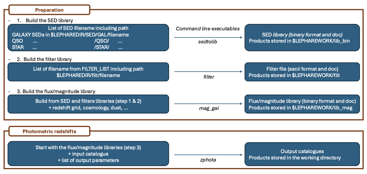
Basic run — Fig. 1 This figure present the four basic steps to run the code with command lines. The steps 1-2-3 could be compressed in a single one using the code “prepare” in python.

Structure of the code

The structure of the package is illustrated in Fig.2.

The executables are stored in your default bin directory when installing the code using pip install. They should be in your PATH and you shouldn’t have to take care of that. If you want to know where the executables are located, try which setolib in your prompt.

If you have installed the code in developper mode, i.e. by cloning the code from the lephare github repository, the C++ source codes are located in LEPHARE/src/lib/ and the python scripts are in LEPHARE/src/lephare/.

Two directories are essential for the functionning of the code:

$LEPHAREDIR is the directory which contains the internal data used by LePHARE, as the filters, the SED templates, the dust attenuation curves, or the opacity of the IGM. If necessary, the user can add new data in this directory (e.g. new filters or new templates).
$LEPHAREWORK is the directory which contains intermediate libraries created by LePHARE. The advantage is that these intermediate libraries don’t need to be created every times you compute the photo-z if they already exist.

These two environment variables could be set in two different ways, depending on your need:

Let the code set these environment variables by default (no action needed on your side). In such case, the code will identify your default cache directory. These directories are indicated in the notebook when excecuting import lephare as lp in a notebook cell.
Set yourself the values of these variables. $LEPHAREWORK could point to any directory you like (intermediate library will be stored inside). $LEPHAREDIR should point to the LePHARE internal data directory (see below).

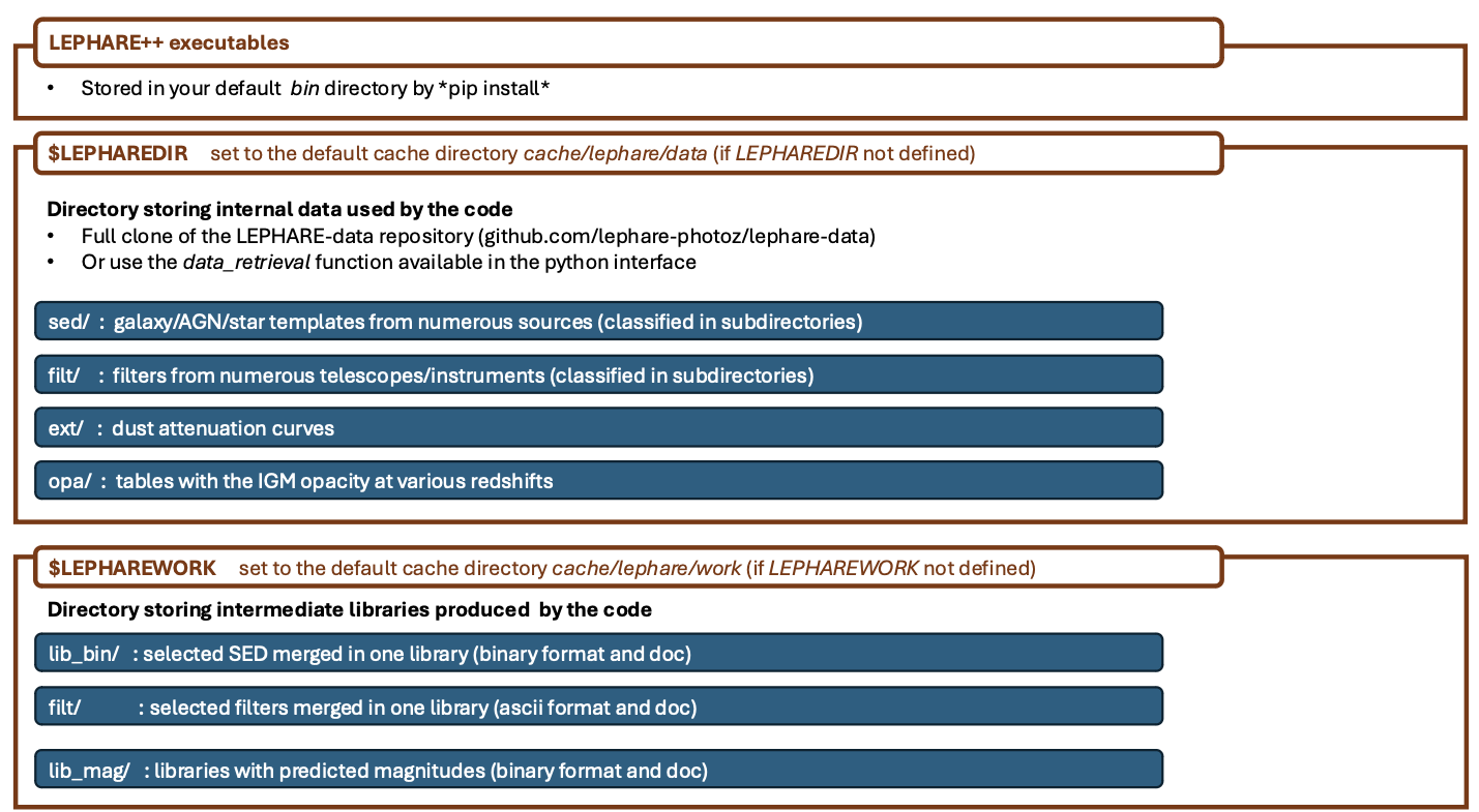
Alternative text — Fig. 2 Structure of the *LePHARE* repository.

The LePHARE internal data directory

The code needs essential information to run, like the filter curves or the SED templates. These informations are stored in one directory which is indicated by the $LEPHAREDIR environment variable. If the user doesn’t set this variable, the code uses by default cache/lephare/data/.

For a question of disk space and downloading time, the internal data are not installed by default. You have different methods to populate this directory:

You can clone the full auxiliary data directory from lephare-data github repository. In such case, the environment variable $LEPHAREDIR should be set to the LEPHARE-data directory path created by the cloning (not done automatically).
You can retrieve all auxiliary data available in LePHARE immediatly, using the function lp.data_retrieval.get_auxiliary_data(clone=True) after having imported lephare as lp in python. You need 2Gb free to download these data. This function allows the user to download only the data needed for the run lp.data_retrieval.get_auxiliary_data(keymap=keymap, additional_files=["examples/COSMOS.in", "examples/output.para"]), with keymap being the map of keywords used to configure the run. The code will check if the data are already stored before downloading them again.

The sub-directories in $LEPHAREDIR are the following:

sed/ which contains three sub-directories for galaxies GAL, for Active Galaxy Nuclei QSO (named QSO for legacy reason), and for stars STAR. Each of these subdirectory contains its own set of templates (the various directories should have a README file and a file named .list with a default list of templates).
filt/ contains subdirectories with telescope/instrument/survey names corresponding to a set of filters. A large number of filters are already included in the package. However, we propose also a solution when using the python interface to download the filters from a Filter Profile Service with a much more extensive filter database.
ext/ includes several dust attenuation curves.
opa/ contains tables with the opacity of the intergalactic medium at various redshifts. The code uses by default the Madau et al. (1995) opacity.
vega/ includes some spectra used for calibration (e.g. Vega to AB convertion).
examples/ includes some parameters files and input files which could be used as an example to run the photo-z on the COSMOS2020 catalogue (Weaver et al. 2022).

The user can add new data in this directory (e.g. if the user want to include a new set of templates not included in LePHARE) following the same model as other files already present in the sub-directories.

Running the code

Configuration files

Two configuration files (noted .para) allow the user to set up the properties of the template-fitting run, as well as the quantitites that the user want in output.

One configuration file set the parameters associated to the run (e.g., $LEPHAREDIR/example/COSMOS.para an example which contains all the keywords). It defines the set of templates, the filters and all the parameters that you want to tune to get the best results. You can save your parameter file where you want (e.g., in the directory where you run the code) to keep configuration files of different runs at any location. Configuration files must be in ASCII format, compliant with the following rules:

Only one parameter per line, with the syntax: PARAMETER_NAME value(s)
Comment line starts with “#”.
Depending on the parameter, values can be Float, Integer, or String (without quotation marks).
When a parameter accepts multiple values, these must be comma separated (no space).
When a parameter accepts a file location (as a String), the path can include environmental variables ($HOME and $LEPHAREDIR).
Some parameters are mandatory. LePHARE will print out an error message if they are not set.
Other parameters can be omitted (LePHARE will assign a default value to them).

In the next sections, we will mark the mandatory parameters with an asterisk (”*”).

A second configuration file (e.g., $LEPHAREDIR/example/output.para) indicates which properties should be written in the output file. The output.para includes all the possible output parameters. You can comment those that are of no intersest to you.

Syntax

with command lines

All the programs in the suite can be run from a Unix shell with the following syntax:

program -c config_file.para \
  -t G \ # type G for Galaxies / only necessary for sedtolib and mag_gal
  --Parameter value \ # optional flag to overwrite

where program is the name of the program (among filter, sedtolib, mag_gal, zphota), followed by a configuration file called with the -c option.

The various code options are defined in the configuration file but can also be given through additional instructions in the command line. Using such an optional list of parameters, any --Parameter value statement overrides the values in the configuration file. All the parameters are listed in the section Keywords.

An extensive example on how to run the code with command lines and including some advanced features is available in this example.

with python

The C++ programs can also be manipulated as a library using the python interface. This is done by importing the LePHARE library in the python scripts or notebooks:

import lephare as lp

Several notebooks are given in example in here.

The detailed run notebook is the closest to the four steps outlined in Fig. 1, i.e. creating the filter library, the SED library, then build the predicted magnitudes from these filters and SEDs (for GAL/QSO/STAR), and finally running the photometric redshifts for a subsample of galaxies from COSMOS2020 having a spec-z.

However, we also added a function lp.prepare which first compute the full predicted magnitude library (the equivalent of combining filter, sedtolib, mag_gal together in the command lines), and then we compute the photometric redshifts with lp.process as in the example below and in this typical run notebook.

# Read the config file within the working directory
config = lp.read_config("your_config.para")
# Example of change in the keywords
config.update(
  {
      "FILTER_FILE": "filter_test",
      "Z_STEP": "0.05,0.,7.",
  }
)
# This line run together all the library preparation
lp.prepare(config)
# Calculate the photometric redshifts
output, pdfs = lp.process(config, input_table)

Build the rest-frame templates library

Overview

In this first step, we generate a unique binary file from different kinds of SEDs (star/AGN/galaxy) with various original formats (ASCII, binary). The binary output file (*.bin) is saved in the directory $LEPHAREWORK/lib_bin/ with an attached doc file (*.doc). An associated file with physical information (*.phys) is provided only for galaxies (not calibrated or not relevant for stars or AGN). For models with input SEDs expressed in luminosity or energy ($L_{\odot}/A$,$\nu L_{\nu}$,…), like BC03, or the FIR libraries, the SED are converted in flux ($erg/s/cm^2/A$).

A set of libraries for stars, galaxies, and AGN are available in $LEPHAREDIR/sed/STAR, $LEPHAREDIR/sed/GAL, $LEPHAREDIR/sed/QSO directories and organized in different sub-folders. Each sub-folder contains a specific collection of SED files, described in a README (how those SEDs were built, etc.), and a file (usually with the suffix .list) listing the relative path of the SED files to be used as input to create the libeary. For STAR and QSO and most of the galaxies, SEDs are written in ASCII, with $\lambda(A)$, flux[$erg/s/A/cm^2$], with increasing $\lambda$. For Galaxy, in addition to empirical SEDs, output files from stellar synthesis population models (BC03) with a more complex format can also be used by adding a specific character BC03 after the file name in the SED list file. Here are two examples of lists with the BC03 templates used in Ilbert et al. (2015) and the COSMOS templates used in Ilbert et al. (2009)

Syntax

with command lines

The program sedtolib is used to build the different STAR, QSO and GAL libraries from a list of SED files.

Specific parameters have been duplicated for the STAR, QSO, and GAL categories with different names to simplify this algorithm section. The option -t allows you to specify if galaxy (G), star (S), or QSO (Q) parameters have to be read. The syntax is

sedtolib -c config_file.para  -t G [or Q or S]

with python

With the python, you need to instantiate an object from the class Sedtolib, and indicate the type of SEDs (GAL/QSO/STAR) when applying the function run.

sedlib = lp.Sedtolib(config_keymap=keymap)
sedlib.run(typ="STAR", star_sed="$LEPHAREDIR/sed/STAR/STAR_MOD_ALL.list")

Parameter values

The parameter value “XXX” means either GAL or QSO or STAR.

parameter	type	default	description
XXX_SED(*)	string (n=1)	—-	Full pathname of file with the list of selected SED files
XXX_LIB(*)	string (n=1)	—-	Name of the output binary library (with no extension). Files $XXX_LIB.bin, $XXX_LIB.doc and $XXX_LIB.phys saved in $LEPHAREWORK/lib_bin/
XXX_FSCALE	float (n=1)	1.0	Flux scale to be applied to each SED in the list
SEL_AGE	string (n=1)	NONE	Full pathname of file with a list of ages (Gyr) to be extracted. Only when using templates including an age (e.g. BC03).
AGE_RANGE	float (n=2)	—–	Range of age (Gyr). Only when using templates including an age (e.g. BC03).

Adding new templates

New SEDs can be easily added to the current ones. They must be located in the appropriate directory (GAL/STAR/QSO) and we also advice to create a subdirectory. If they are ASCII files they must be in $\lambda(A)$, flux[$erg/s/A/cm^2$], with increasing $\lambda$.

Output

The binary output file (*.bin) is saved in the directory $LEPHAREWORK/lib_bin/ with an attached doc file (*.doc) and a file with physical information (*.phys) for galaxies.

Others

Already included libraries

The easiest is to take a predefined list of SED in the existing subdirectories and look at the README file.

For stars ($LEPHAREDIR/sed/STAR), SEDs are available in the subdirectories :

PICKLES/: 131 stellar SEDs from Pickles (1998)
BD/: Low mass stars library from Chabrier et al. (2000)
BD_NEW/: Brown dwarfs library from Baraffe et al. 2015, Morley et al. 2012, 2014
LAGET/: (missing REF)
WD/: 4 white dwarfs from Bohlin et al. (1995)
SPEC_PHOT: Spectro-Photometric standards from Hamuy et al. (1992, 1994)

For AGN ($LEPHAREDIR/sed/QSO), there is a list of observed spectra from different authors and some synthetical AGN listed in the subdirectory. In particular, a list of templates was successfully used for computing the photometric redshift of the XMM and Chandra AGN identified in COSMOS. In short, the library includes pure QSO and hybrid templates obtained by combining galaxies with various AGN and QSO templates with different relative ratios. The details of the template construction are outlined in Salvato et al. (2009). Note that, unlike for galaxies, the templates to be used in QSO depend on the type of AGN and QSO to be fitted (see Salvato et al 2011, Fotopoulou et al. 2012, Hsu et al. 2014, Ananna et al. 2017)

For galaxies ($LEPHAREDIR/sed/GAL), SEDs are available in the following subdirectories:

CFHTLS_SED/: 66 SEDs used for CFHTLS photo-z paper (Arnouts et al. 2007)
COSMOS_SED/: 31 SEDs used for COSMOS photo-z paper (Ilbert et al. 2009, 2013, Salvato et al. 2011, Dahlen et al. 2013)
CWW_KINNEY/: original CWW and Kinney spectra
BC03_CHAB/: SEDs from the BC03 library. These templates are derived with exponentially declining Star Formation Histories.
BC03_CHAB_DELAYED/: SEDs from the BC03 library. These templates are derived with delayed Star Formation Histories.

For Far-Infrared (FIR) SEDs ($LEPHAREDIR/sed/GAL), different SEDs are available :

CHARY_ELBAZ/: 105 FIR templates for different luminosity
DALE/ : 64 FIR templates
LAGACHE/: 46 FIR templates
SK06/ : different set of starburst models based on Siebenmorgen &Krugel (2006)

Note

Note that for the first 3 libraries (CHARY-ELBAZ, DALE, LAGACHE), we have subtracted a stellar component from their SEDs to get only the dust contribution at the shortest wavelengths.

To know the format of the SEDs that are used in your list, an additional character must be specified after each SED file, allowing you to mix in one list of different types of galaxy SEDs. For example, you could prepare a new list which includes:

BC03_CHAB/bc2003_lr_m52_chab_tau03_dust00.ised_ASCII BC03
BC03_CHAB/bc2003_lr_m62_chab_tau03_dust00.ised_ASCII BC03
COSMOS_SED/Ell1_A_0.sed
COSMOS_SED/Ell2_A_0.sed

In each list, it is possible to comment out a template with #. For ASCII SED file, no character is required. The character BC03 is used for the Bruzual and Charlot 2003 models. For the BC03 templates, the files are in ASCII for the C++ version of LePhare, to avoid the problem of portability between various systems.

For the list with FIR SEDs, the character LW (as for Long Wavelength) is required, with an example for Chary and Elbaz (2001) templates list.

Find physical information associated to the library

For the galaxy templates, an additional file is generated associated to the library. The file $LEPHAREWORK/lib_bin/*.phys contains the following parameters:

Model Age $L_{UV}$ $L_R$ $L_K$ $L_{IR}$ Mass SFR Metallicity Tau $D_{4000}$

where
Age is expressed in yr
\(L_{UV}\) is near-ultraviolet monochromatic luminosity (Log([erg/s/Hz])) (\(\int_{2100}^{2500} L_{\lambda} d\lambda /400 * 2300^2/c\) ))
\(L_R\) is optical r monochromatic luminosity (Log([erg/s/Hz]))  (\(\int_{5500}^{6500} L_{\lambda} d\lambda /1000 * 6000^2/c\) ))
\(L_K\) is near-infrared K monochromatic luminosity (Log([erg/s/Hz]))  (\(\int_{21000}^{23000} L_{\lambda} d\lambda /2000 * 22000^2/c\)  ))
\(L_{IR}\) is the infrared luminosity (Log([\(L_{\odot}\)]))
Mass is the stellar mass (\(M_{\odot}\)), .i.e. the mass truly in  stars (not the integral of the SFH)
SFR is the ongoing star formation rate (\(M_{\odot}/yr\))
Metallicity is the Gas metallicity of the galaxy
Tau is the e-folding parameter for a star formation history with  SFH=exp(-t/tau) (yr)
\(D_{4000}\) is the 4000A break measured as in Bruzual 1983 (\(D_{4000}= \int_{4050}^{4250} F_{\lambda} d\lambda / \int_{3750}^{3950} F_{\lambda} d\lambda\))

If not available, the parameters are set to -99.

The IR luminosity ($L_{IR}$) is derived using LW libraries (LW for Long Wavelengtgh to describe the dust emission). For the Infra-red libraries ( LW: Dale, Lagache, Chary-Elbaz, Siebenmorgen & Krugel) the IR luminosity is measured from 8 to 1000 microns. These luminosities may be slightly different then the ones quoted by the authors due to the different definitions of the $L_{IR}$ integration limit and because (at least for Dale, Lagache, and Chary-Elbaz) we have subtracted the underlying stellar component from the original SEDs.

Build the filter library

Overview

The goal of this step is to:

read a list of filter, corresponding to the ones used in your input catalogue;
read each of these filters and convert them into a common format;
store them in a common library in $LEPHAREWORK/filt/.

Several sets of filters from different telescopes/instruments are available in the directory $LEPHAREDIR/filt/. You could find in this directory most of the standard filters (like the Johnson-Kron-Cousins in filt/jkc). In order to know the existing filters in lephare-data, the simplest is to look at https://github.com/lephare-photoz/lephare-data/tree/main/filt, or the directory lephare-data if everything was cloned. The filters will be downloaded automatically if a clone of the full lephare-data wasn’t done.

You could also store new filters in another directory than $LEPHAREDIR/filt/ using the keyword FILTER_REP.

Syntax

with command lines

The program filter puts together a list of filter response curves, and applies some transformations according to the nature of the filters as define in the configuration file.

filter -c config_file.para

The resulting file is placed in the directory $LEPHAREWORK/filt/.

with python

With the python interface, you need to instantiate an object from the class Filter, and apply the function run.

filterLib = lp.Filter(config_file=config_file)
filterLib.run()

Parameter descriptions

Parameters	type	default	description
FILTER_REP	string (n=1)	$LEPHAREDIR/filt/	Name of the repository containing the filters.
FILTER_LIST	string Nfilt not limited	—-	filter files separated by a comma. Keep the same order as in the input photometric catalogue.
TRANS_TYPE	float n=1 or n=Nfilt	0	Filter transmission type: 0= Energy; 1= Photon
FILTER_CALIB	integer n=1 or n=Nfilt	0	Filter calibration for long wavelengths [0-def]. Could use a value per filter separated with coma.
FILTER_FILE	string (n=1)	filter	Name of the output file with all combined filters . It is saved in $LEPHAREWORK/filt/

FILTER_LIST: all the filter names must be separated by a comma. We assume that all the filter files are located in the directory $LEPHAREDIR/filt/, except if the keyword FILTER_REP is specified. When writing the set of filters to be used, only the pathname after the common string $LEPHAREDIR/filt/ should be specified.

TRANS_TYPE: type of the transmission curve for each filter, separated by a comma. The number of arguments should match the number of filter, unless only one is given. In that case it will be used for all filters. The transmissions ($T_{\lambda}$) are dimensionless (in % ), however they refer either to a transmission in Energy or Photon which will slightly modify the magnitude estimates. The magnitude is :

\[mag(*) = -2.5 \log_{10} \frac{\int F_{\lambda}(*) R_{\lambda} d\lambda}{\int F_{\lambda}(Vega) R_{\lambda} d\lambda}\]

If the transmission curve ($T_{\lambda}$) corresponds to energy then $R_{\lambda}=T_{\lambda}$. If the transmission curve ($T_{\lambda}$) corresponds to number of photons ($N_{\varphi}$) then $R_{\lambda}= \lambda T_{\lambda}$ :

\[N_{\varphi} = \frac{ F_{\lambda} d\lambda }{h\ \nu} = \frac{F_{\lambda} \lambda d\lambda }{h\ c} \rightarrow mag(*)=-2.5 \log_{10} \frac{\int F_{\lambda}(*) \lambda T_{\lambda} d\lambda}{\int F_{\lambda}(Vega) \lambda T_{\lambda} d\lambda} \rightarrow R_{\lambda}=\lambda T_{\lambda}\]

When building the filter library, the filter shape is changed with respect to the original one as follows :

\[R_{\lambda}=T_{\lambda} ( \frac{\lambda}{< \lambda >})^{tt}\]

where $tt$ is the value of TRANS_TYPE parameter and $< \lambda >$ is the mean wavelength of the filter. The modification of filter shape can be significant for long wavelength filters and when the filter is broad. Nevertheless it is often not the dominant source of errors with respect to other uncertainties relative to QE-CCD, telescope transmission, atmospheric extinction shape etc…

In the output filter file specified by the keyword FILTER_FILE, we save the values ($\lambda (A)$,$R_{\lambda}$).

FILTER_CALIB: This keyword allow to consider specific calibrations at long wavelengths in order to apply a correction factor to the original flux estimated by LEPHARE. We define the correction factor as fac_corr$=\frac{\int R_{\nu} d\nu}{\int \frac{B_{\nu}}{B_{\nu_0}} R_{\nu} d\nu}= \frac{\int R_{\lambda} d\lambda/\lambda^2}{1/\lambda_0^2 \int \frac{B_{\lambda}}{B_{\lambda_0}} R_{\lambda} d\lambda}$, where $B_{\nu}$ is the reference spectrum used to calibrate the filters and $\lambda_0$ is the effective wavelength defined as $\lambda_{0}= \frac{\int R_{\lambda} B_{\lambda} \lambda d\lambda}{\int R_{\lambda} B_{\lambda} d\lambda}$. The value of FILTER_CALIB allows to describe different combinations of $\nu_0$ and $B_{\nu}$:

FILTER_CALIB=0 \(\frac{B_{\nu}}{B_{\nu_0}}=1\) or \(B_{\nu}=ctt\). This is the default value used in LePHARE.
FILTER_CALIB=1 \(\nu B_{\nu}=ctt\). This describes the SPITZER/IRAC, ISO calibrations.
FILTER_CALIB=2 \(B_{\nu}=\nu\). This describes the sub-mm calibrations.
FILTER_CALIB=3 \(B_{\nu}=\)black body at T=10,000K.
FILTER_CALIB=4 : A mix calibration with \(\nu_0\) defined from \(\nu B_{\nu}=ctt\) and the flux estimated as \(B_{\nu}=\)black body at T=10,000K. This appears to be the adopted scheme for the SPITZER/MIPS calibration.
FILTER_CALIB=5 : Similar mix calibration with \(\nu_0\) defined from \(\nu B_{\nu}=ctt\) and the flux estimated as \(B_{\nu}=\nu\). This may reflect the SCUBA calibration.

Adding a new filter

In general

Filters are ASCII files with the following format : | In first row : # SHORT_NAME_of_FILTER ADD_COMMENTS | In next rows : $\lambda (A)$ Transmission

Wavelengths must be in increasing order. It is better to put the lowest and highest $\lambda$ with Transmission=0. The units of transmission are not considered.

The header, the transmission at 0 on the edges, and the transmission sorted in lambda are set internally if not prepared by the user.

As an exemple : filter pippo.pb and put it in $LEPHAREDIR/filt/pippo/pippo.pb :

# PIPPO	This is close to window function
5000	0
5001	1
5999	1
6000	0

The user should avoid setting a resolution that is unnecessarily high, as this could result in expensive computational time for the predicted magnitude library.

Getting new filter automatically (only in python)

The python interface allows to load the filters from a yml file, with the possibility to query the SVO service including a much larger number of filters.

filterLibSVO = lp.FilterSvc.from_yaml(f"{lp.LEPHAREDIR}/examples/config_svo_filters.yml")
filter_output = os.path.join(os.environ["LEPHAREWORK"], "filt", keymap["FILTER_FILE"].value)
lp.write_output_filter(filter_output + "_svo.dat", filter_output + "_svo.doc", filterLibSVO)

where $LEPHAREDIR/examples/config_svo_filters.yml is a yml file including the name of filters to be downloaded. You can copy the yaml file into your own directory and modify the names of the filters according to the ones in the SVO website. The transmission type is given in the SVO webpage. The filters will be stored in LEPHAREWORK/filt/ and name defined according to the keyword FILTER_FILE.

Output

The filters are stored in a single ascii file as given by FILTER_FILE and store in $LEPHAREWORK/filt/ with an attached doc file (*.doc).

Additionnal features

Get information on the filters

As an example, using default values listed in the configuration file zphot.para.

FILTER_LIST	tmp/f300.pb,tmp/f450.pb, tmp/f606.pb,tmp/f814.pb,tmp/Jbb.pb,tmp/H.pb,tmp/K.pb
TRANS_TYPE	0
FILTER_CALIB	0
FILTER_FILE	HDF.filt

When building the filter library, the following informations are written on the screen :

#NAME	ID	$\lambda_{eff}^{mean}$	$\lambda_{eff}^{Vega}$	FWHM	ABcor	TGcor	VEGA	$M_{\odot}^{AB}$	CAL	$\lambda_{0}$	Fac
F300W	1	0.2999	0.2993	0.0864	1.398	99.99	-21.152	7.433	0	0.2999	1.000
F450W	2	0.4573	0.4513	0.1077	-0.074	-0.339	-20.609	5.255	0	0.4573	1.000
F606W	3	0.6028	0.5827	0.2034	0.095	0.161	-21.367	4.720	0	0.6028	1.000
F814W	4	0.8013	0.7864	0.1373	0.417	0.641	-22.322	4.529	0	0.8013	1.000
Jbb	5	1.2370	1.2212	0.2065	0.890	99.99	-23.748	4.559	0	1.2370	1.000
H	6	1.6460	1.6252	0.3377	1.361	99.99	-24.839	4.702	0	1.6460	1.000
K	7	2.2210	2.1971	0.3967	1.881	99.99	-26.012	5.178	0	2.2210	1.000

where :
Col 1 : Name put in the first row of the filter file
Col 2 : incremental number
Col 3 : Mean wavelength (\(\mu m\)) : \(\int R_{\lambda} \lambda d\lambda / \int R_{\lambda} d\lambda\)
Col 4 : Effective wavelength with Vega (\(\mu m\)) : \(\int R_{\lambda} F_{\lambda}(Vega)\lambda d\lambda / \int R_{\lambda}F_{\lambda}(Vega) d\lambda\)
Col 5 : Full Width at Half of Maximum (\(\mu m\))
Col 6 : AB Correction where \(m_{AB} = m_{VEGA} + ABcor\)
Col 7 : Thuan Gunn correction where \(m_{TG} = m_{VEGA} + TGcor\). (99.99 if undefined)
Col 8 : VEGA magnitude : \(2.5\log_{10}(\int R_{\lambda} F_{\lambda}(Vega) d\lambda / \int R_{\lambda} d\lambda\))
Col 9 : AB absolute magnitude of the sun (\(M^{AB}_{\nu,\odot}\))
Col 10: value of the calibration used for (\(B_{\nu}/B_{\nu_0}\),\(\nu_0\)) in FILTER_CALIB
Col 11: Effective wavelength (\(\mu m\)) \(\lambda_{0}^{B_{\nu}}= \frac{\int R_{\lambda} B_{\lambda} \lambda d\lambda}{\int R_{\lambda}  B_{\lambda}  d\lambda}\).
Col 12: Correction factor to be applied to the original flux measured by LEPHARE. This correction is included in the programs mag_gal and mag_star as \(flux^{cor}= flux^{LePhare}\times\)fac_cor

Extinction informations

The stand alone program (filter_extinc) returns information about
atmospheric extinctions and galactic extinctions.
A set of atmospheric extinction curves and galactic extinction laws
are available in $LEPHAREDIR/ext/ directory. It includes Calzetti and
Prevot extinction laws. The Cardelli law is hardcoded in the programs
and is the default law for the galactic extinction.
% filter_extinc -c COSMOS.para -FILTER_FILE filter_test.dat
It returns:
# Computing ATMOSPHERIC AND GALACTIC EXTINCTIONS
# with the following options:

# Filters:	filter_extinc.dat
# Atmospheric extinction curve:	extinc_etc.dat
# Galactic extinction curve:	CARDELLI
# Output file:	filter_extinc.dat

Filters	Ext(mag/airmass)	Albda/Av	Albda/E(B-V)
cosmos/u_cfht	0.486	1.504	4.663
cosmos/B_subaru	0.264	1.297	4.020
cosmos/V_subaru	0.141	1.006	3.118
cosmos/r_subaru	0.096	0.858	2.659
cosmos/i_subaru	0.052	0.643	1.992
cosmos/suprime_FDCCD_z	0.027	0.471	1.461
vista/Y	0.049	0.391	1.211
vista/J	0.096	0.281	0.871
vista/H	0.100	0.181	0.562
vista/K	0.100	0.118	0.364

Col 2 : Mean atmospheric extinction (mag/airmass) using (EXT_CURVE):
\(A_{\lambda}= \int R_{\lambda} Ext(\lambda) d\lambda / \int R_{\lambda} d\lambda\)
\(Ext(\lambda)\) comes from any atmospheric extinction curve that
is put in $LEPHAREDIR/ext/.
Col 3 : Mean galactic attenuation (in \(A(\lambda)/A_V\)) using
the galactic extinction law (GAL_CURVE). Col 4 : Mean galactic
attenuation (in \(A(\lambda)//E(B-V)\)) as a function of color
excess (E(B-V)) assuming \(A_V=R_V\times E(B-V)\).
For \(R_V\) coefficients, we assume \(R_V=3.1\) for most
extinction laws but Calzetti (\(R_V=4.05\)) and Prevost
(\(R_V=2.72\)).
Others extinction laws can be added by following the format
(\(\lambda(A) , k_{\lambda}\)).

Application to long wavelengths

LePHARE has been developped for the optical-NIR domain but can be used at shorter (UV) and longer wavelengths (FIR, submm and radio). In particular extensive tests have been performed in the long wavelength domain by E. Le Floc’h to evaluate the photometric accuracy. Some issues have to be considered :

the Vega spectrum is not defined at $\lambda\ge 160\mu m$. Thus, the AB magnitude system should be used as standard when combining a large wavelength domain.
The bandpass in radio domain is very narrow and does not require to convolve through the filter. However the structure of LePHARE requires to implement a transmission curves for the radio frequencies in similar way as in shorter wavelengths.

More important, at long wavelengths the equivalent fluxes are taken as the monochromatic flux density calculated at the effective wavelength of the filter and for a reference spectrum that would result in the same energy received on the detector:

\[<F_{\nu}> = \frac{\int F_{\nu} R_{\nu} d\nu}{\int \frac{B_{\nu}}{B_{\nu_0}} R_{\nu} d\nu}\]

where $B_\nu$ is the reference spectrum and $\nu_0$ the effective frequency of the filter. In LePHARE, the flux estimates are equivalent to consider $\frac{B_{\nu}}{B_{\nu_0}}=1$ ($B_{\nu}=ctt$). Therefore there is a correction factor to account for with respect to the original flux estimated by LePHARE. This correction is :

\[<F_{\nu}>^{COR} = <F_{\nu}>^{LePhare} \times \frac{\int R_{\nu} d\nu}{\int \frac{B_{\nu}}{B_{\nu_0}} R_{\nu} d\nu}\]

At long wavelengths, different conventions have been used for the
reference spectrum. As an example: SPITZER/IRAC uses a flat spectrum
(\(\nu B_{\nu}=ctt\)) as well as ISO; SPITZER/MIPS uses a
blackbody with temperature T=10000K while SCUBA uses planets which
have SEDs in submillimeter very close to \(B_{\nu}=\nu\). The
keyword FILTER_CALIB is used to account for these different
calibration scheme (see Build the filter library).
One additional effect is the way the effective wavelength is defined.
In the case of MIPS, the effective wavelength seems to be defined,
according to the MIPS handbook, as \(\nu B_{\nu}=ctt\) while the
reference spectrum is a black body. This mix definition can be
described with FILTER_CALIB=4.
In the table below we report the effective wavelengths and the
correction factors that are applied to LEPHARE fluxes for a set of
filters spanning from NIR (K band), MIR (SPITZER/IRAC), FIR
(SPITZER/MIPS), sub-mm (SCUBA) to radio (VLA: 1.4GHz).

#NAME	$\lambda_{mean}$	$M_{\odot}^{AB}$	CAL	$\lambda_{0}^{B_{\nu}}$	Fac	CAL	$\lambda_{0}^{B_{\nu}}$	Fac
K	2.2210	5.178	0	2.2210	1.000	0	2.2210	1.000
IRAC_1	3.5634	6.061	1	3.5504	1.004	1	3.5504	1.004
IRAC_2	4.5110	6.559	1	4.4930	1.004	1	4.4930	1.004
IRAC_3	5.7593	7.038	1	5.7308	1.005	1	5.7308	1.005
IRAC_4	7.9595	7.647	1	7.8723	1.011	1	7.8723	1.011
24mic	23.8437	9.540	4	23.6750	0.968	3	23.2129	1.006
70mic	72.5579	12.213	4	71.4211	0.932	3	68.4725	1.013
160mic	156.9636	13.998	4	155.8945	0.966	3	152.6311	1.007
850mi	866.7652	nan	5	865.3377	0.997	2	862.4710	1.000
VLA_1.4GHz	214300	nan	5	214248.3782	1.000	2	214145.1645	1.000

As can be seen from this table :
\(\bullet\) For K band, we use FILTER_CALIB=0, so no correcting
factor is applied.
\(\bullet\) For IRAC bands , we adopt \(\nu B_{\nu}=ctt\)
(FILTER_CALIB=1). The correction factors are less than 1% and can be
neglected.
\(\bullet\) For MIPS bands (24, 70, 160\(\mu m\)), we adopt
\(B_{\nu}=BB(T=10,000K)\) and \(\lambda_0\) defined as
\(\nu B_ {\nu}=ctt\) (FILTER_CALIB=4), which seems to better
reflect the current MIPS calibration. In this case, correction factors
between 3% to 7% are applied to the magnitudes predicted from the templates. However, we also compare the correction
factors when both \(\lambda_0\) and \(B_{\nu}\) refer to a
black body at T=10,000K (FILTER_CALIB=3). In this case, the
corrections become negligeable with \(\sim\)1%.
\(\bullet\) For sub-mm (SCUBA, 850\(\mu m\)) and radio (VLA:
1.4GHz) wavelengths, no correction is required
As a general conclusion, the flux measured by LEPHARE appear accurate
at a level of 1% with respect to most of the calibration scheme
considered at long wavelength and thus no correction is required. A
special warning for MIPS calibration, where depending on the
calibration scheme, a correction up to 7%, may be applied to the predicted magnitudes when computed.

Build the predicted flux/magnitude library

Overview

In this step, the program predicts the magnitudes expected for GAL/QSO/STAR templates integrated through the filter curves along a grid of redshifts. It establishes the predicted flux/magnitude library which will be compared later to the data.

Syntax

with command lines

The program mag_gal is used to build the different STAR, QSO and GAL predicted magnitude/flux libraries. The option -t allows you to specify if galaxy (G), star (S), or QSO (Q) parameters have to be read. The syntax is:

mag_gal -c config_file.para  -t G [or Q or S]

with python

You need to instantiate an object from the class MagGal, and indicate the type (GAL/QSO/STAR) when applying the function run.

maglib = lp.MagGal(config_keymap=keymap)
maglib.run(typ="GAL",gal_lib_in="LIB_GAL",gal_lib_out="VISTA_COSMOS")

Parameter values

For a set of filters given by FILTER_FILE and an input SED library defined by GAL_LIB_IN, the magnitudes are computed at different redshifts defined by Z_STEP. Extinctions can be applied as specified by the three keywords (EXTINC_LAW, MOD_EXTINC, EB_V). If evolving stellar population models are used, the cosmology (COSMOLOGY) will allow to reject models older than the age of the universe. The magnitude in VEGA or AB (defined by MAGTYPE) are saved in the binary file defined by GAL_LIB_OUT in $LEPHAREWORK/lib_mag/ with an attached doc file. An output file (LIB_ASCII YES) is written to check the magnitudes, color tracks with redshift.

Parameters	type	default	description
FILTER_FILE(*)	string (n=1)	—-	Name of the filter file. File must already exist in $LEPHAREWORK/filt/
XXX_LIB_IN(*)	string (n=1)	—-	Name of the GAL/QSO/STAR binary library (with no extension). Files must already exist in $LEPHAREWORK/lib_bin/
XXX_LIB_OUT(*)	string (n=1)	—-	Name of the magnitude binary library (with no extension). Files created as GAL[QSO]_LIB_OUT*.bin (.doc) and saved in $LEPHAREWORK/lib_mag/
MAGTYPE(*)	string	—-	Magnitude type (AB or VEGA)
Z_STEP	float (n=3)	0.04,0,6	dz,zmin,zmax: redshift step, dz dz constant step in redshift The minimum (zmin) and the maximum redshift (zmax).
COSMOLOGY(*)	float (n=3)	—-	$H_0$, $\Omega_0$, $\Lambda_0$. Used for age constraints.
EXTINC_LAW	string (n $\le$ 10)	NONE	Extinction laws to be used (in $LEPHAREDIR/ext/) several files separated by comma
MOD_EXTINC	integer (n $\le$ 20)	0,0	Range of models for which extinction will be applied. The numbers refer to the models in the $GAL_SED list
			Number of values must be twice the number of extinction laws.
EB_V	float		Reddening color excess E(B-V) values to be applied
	(n $\le$ 100)		values separated by comma.
EM_LINES	string (n=1)	NO	Add contribution of emission lines and specify how to derive them (`EMP_UV`, `EMP_SFR`, `PHYS`). Only applied to galaxy templates
EM_DISPERSION	float	1	the emission lines can vary by these fractions from the expected value (example 0.5,1.,1.5)
ADD_DUSTEM	string	NO (n=1)	Add the dust emission in templates when missing. This is based on the energy absorbed over the UV-optical range.
LIB_ASCII	string (n=1)	NO	ASCII file with magnitudes saved in $LEPHAREWORK and called $GAL[QSO]_LIB_OUT.dat

The extinction laws and dust emission

A set of extinction (or attenuation) laws are available in the directory ($LEPHAREDIR/ext/). Several extinction laws can be used at the same time and set up in the keyword EXTINC_LAW. Each extinction law will be applied to a range of SED models specified by the keywords MOD_EXTINC. The model number corresponds to the rank in the list of SEDs used in GAL_SED. For each extinction law, two numbers needs to be provided indicating the first and last model number of a range. So, the number of models must be twice the number of extinction laws. For instance, if EXTINC_LAW SMC_prevot.dat,SB_calzetti.dat, we expect four numbers for MOD_EXTINC 13,23,23,31 with the first law applied to the model between 13 and 23, and the second law between 23 and 31.

The different values of reddening excess E(B-V) are given in the keyword EB_V and will apply to all extinction laws. The extinguished flux is : $F_{\lambda}^e = F_{\lambda}^0\ 10^{-0.4 A_{\lambda}}= F_{\lambda}^0\ 10^{-0.4 k_{\lambda} E(B-V)}$

If dust extinction is applied, a prediction of the expected IR dust luminosity is computed using energy balance.

Some templates don’t include dust emission, as for instance BC03 (or any template extrapolated in infrared using CSP models). We add the possibility of having the dust emission by using ADD_DUSTEM YES using this energy balance principle. In such case, we use the templates from Bethermin et al. (2012) (hereafter B12) and sum their flux contribution to the stellar template (e.g. BC03). Don’t use this option if your templates already include dust emission. The B12 templates are different for each redshift, as given in the B12 list. However, a current limitation of the code is that we can display only the first template of the list in FIR in the .spec file, while we use the correct redshifted template when we do the fit. This limitation affect only the display of the .spec file in FIR. But to avoid confusion, we limit ourself to only one B12 template in the list. You can decide to remove the comments in front of the other B12 templates and use all of them, knowing that the display could be affected (but the internal fit correct).

The Emission lines

The role of nebular emission lines is essential when using medium-bands (Ilbert et 2009), but also when using only broad-band filters (Schearer et al. 2009, Labbe et al. 2013, Stefanon et al. 2015). Some galaxy templates already include emission lines. In this case, you could use EM_LINES NO to avoid creating additional ones. To include emission lines in the template galaxy SEDs if they don’t exist, one of the available methods must be selected through the parameter EM_LINES. There are three different options:

EMP_UV LePHARE accounts for the contribution of emission lines with a simple recipe based on the Kennicutt (1998) relations. The SFR is estimated from UV luminosity, which in turn defines the H$\alpha$ luminosity. Intensity of other lines ($Ly_{\alpha}$, $H_{\alpha}$, $H_{\beta}$, [OII], OIII[4959] and OIII[5007]) are defined accordingly by using the flux ratios provided in Ilbert et al. (2009) and slightly adjusted since. The UV luminosity is derived directly from the SED template. Emission lines are not considered in red galaxies with $(NUV-r)_{ABS}\ge 4$ (rest frame, dust corrected color). This option works for any kind of input template.
EMP_SFR At present, this option can be used only with BC03 templates. This option can be used with SED templates that have SFR already defined (BC03). The SFR is converted in H$\alpha$ according to Kennicutt (1998). It skips the conversion from UV to SFR done with the option EMP_UV.
PHYS At present, this option can be used only with BC03 templates. For each of them, LePhare reads metallicity, fraction of photoionizing photons, and other physical quantities needed as input in a model (Schearer et al. 2009) that quantifies flux emitted by several emission lines. To see details and applications of this method in Shun et al. (2019, in prep).

In all the methods, dust attenuation is applied to the emission line according the continuum value. The MW (Seaton 1979) extinction curve is considered for the emission lines. A factor $f$ is introduce between the E(B-V) obtained for the stellar content and the E(B-V) considered for the emission lines. This value is taken as 1.

With the option EM_DISPERSION, the emission lines can vary from the standard value; for example by setting the option to EM_DISPERSION 0.5,1.,1.5 the code generates three SEDs with identical characteristics, except the lines will have the standard flux (prescribed by the EMP_ or PHY recipe) and $\pm50\%$ of that value.

Even if emission lines have been built for the entire library, during any SED fitting run the user can decide to ignore them for a given subset of models (see ADD_EMLINES option).

This option is not appropriated for the AGN samples. For AGN, the contribution from emission lines to the flux in a given band is even stronger than for normal galaxies. Do not compute emission lines using star-formation recipes established for galaxies. The templates in QSO are empirical (e.g. Salvato et al. 2009,….) and thus the emission lines are already included in the SED. For the syntethic models of QSO included in QSO/SYNTH the emission lines are also already included.

Outputs

The binary output file (*.bin) is saved in the directory $LEPHAREWORK/lib_mag/ with an attached doc file (*.doc).

An output file is produced in the current directory if LIB_ASCII YES. It has the same root name as the binary file with extension .dat and contains the following informations :

Model, Extinc-law, E(B-V), $L_{TIR}(L_{\odot})$, Z, DMod, Age(yr), nrec, n , (mag(i),i=1,n),(kcor(i),i=1,n)

where Model is the number of models based on the original list, Extinc-law refers to the number of the extinction laws used, $L_{TIR}$ the new estimate of the IR luminosity, DMod is the distance modulus, nrec is a record (internal use), n the number of filters, mag(i) the predicted magnitudes in all filters and kcor(i), the k-correction in all filters (see Hogg 1999 for definitions).

You must be aware that the size of the library becomes quickly huge if you do not pay attention. You can estimate its size by considering the following numbers : # of models x # of age x # of z steps x # of extinction law x # of EB-V. For exemple, 10 SEDs with 60 ages, 2 extinction laws and 6 E(B-V) and 150 z steps will exceed 1,000,000 rows.

Compute photometric redshifts

Overview

The final step performs a $\chi^2$-based analysis, fitting the predicted flux built previously to the observed photometry (AB/Vega magnitudes or fluxes). To measure the photometric redshift, we use a $\chi^2$ fitting procedure by comparing the observed flux ($F_{obs}$) and its corresponding uncertainties ($\sigma$) with the flux from templates ($F_{temp}$) defined as:

\[\chi^2 = \sum_i [ \frac{F_{obs,i} - s F_{temp,i}}{\sigma_i}]^2\]

where i refers to the band used for the analysis and $s$ the scaling factor that is chosen to minimize the $\chi^2$ values (${\it d}\chi^2/{\it d}s=0$):

\[s = \sum_j [ \frac{F_{obs,j} F_{temp,j}}{\sigma_j^2} ] / \sum_j [ \frac{F_{temp,j}^2}{ \sigma_j^2}]\]

where j refers to the band used for the scaling (j can be different from i). The photometric baseline can span a large wavelength range, as long as the templates are established accordingly. Galaxy, star, and QSO libraries can be used in the same run, but the $\chi^2$ minimization process is performed distinctly for each class. For a given class (e.g., galaxy SEDs) several libraries can be combined.

Different options are available to improve the $z_\mathrm{phot}$ measurement: physical priors, adaptive photometric adjustments, addition of nebular emission lines in the synthetic SEDs. If the templates include physical information (e.g. BC03), the code can output the stellar mass, star formation rate, etc., for each object.

Syntax

Note: you should use the option VERBOSE NO if you run in batch mode.

With command lines

The program zphota is used to derive the photo-z and the physical parameters.

zphota -c config_file.para --CAT_IN sourcelist.in

with sourcelist.in being the input file in ascii format with command lines (an advantage with the python interface is that you can use any format).

With python

You can run the photometric redshift with the function lp.process prepared to facilitate your work, or using the class lp.PhotoZ. Here are the two methods:

# Read the config file within the working directory
config = lp.read_config("zphot.para")
# This line run together all the library preparation
lp.prepare(config)
# Calculate the photometric redshifts
output, pdfs = lp.process(config, input_table)

The input_table is a python table with a pre-defined format (explained below).

# Instantiate an object from the class ``PhotoZ``
photz = lp.PhotoZ(keymap)
# Fit
photz.run_photoz(sourcelist, [],[] )

The sourcelist is a vector of objects of the class onesource containing all the necessary input information (e.g. fluxes, magnitudes, …).

Input

This section describes how to manage the input file. The associated keywords are listed here. Most of them become useless when using the python interface.

Input catalog

Parameters

Type

Default val.

Description

CAT_IN(*)

string[1]

—-

Name of the input photometric catalogue (full path)

INP_TYPE(*)

string[1]

—-

Input values: Flux (F) or Magnitude (M);

CAT_MAG(*)

string[1]

—-

Input magnitude type : AB or VEGA

CAT_FMT(*)

string[1]

—-

Input format for photometry (MEME or MMEE)

CAT_LINES

integer[2]

-99,-99

Min and max rows read in input catalog (starting from 1). Read all the catalogue by default

CAT_TYPE

string[1]

SHORT

Input catalog format

The information needed for the fit

We expect in input:

an identification number (Id);
the apparent magnitudes (or fluxes);
the corresponding errors.
A Context value associated to each source indicates which passbands can be used for the object, explained in Context
$z_\mathrm{spec}$ is the input redshift (can be also equal to -99 if not defined).

The filters in the input catalog must be the same and in the same order as in the predicted magnitude library (the one stored in $LEPHAREWORK/lib_mag).

Context and $z_\mathrm{spec}$ are only compulsory in the LONG format. Context could be set at 0 to consider all filters.

For a given object, the magnitude (or flux) in a given filter could miss (not observed or the photometric extraction failed). If the magnitude (or flux) and the associated are both negative, this filter will be ignored (for instance, you can put -99 -99 for the flux and associated error). This is another way to ignore a band than context.

If the measurement is missing because the flux is too faint to be detected, one could use an upper-limit. In such case, the magnitude (or flux) are positive and set to the upper-limit value while the error should be negative. The predicted magnitude will be forced to be fainter than the magnitude given in the photometric catalogue. We advice to use flux with appropriate uncertainties and no upper-limits, which is more correct statistically.

The input catalogue could include magnitudes or fluxes. To use fluxes, you must specify F for the parameter INP_TYPE and fluxes must be given in $\mathrm{erg}/\mathrm{s}/\mathrm{cm}^2/\mathrm{Hz}$. If you use magnitude in input, use INP_TYPE M. In this case, The calibration system is declared by the parameter CAT_MAG, which can be either VEGA or AB.

Input file when using command lines

We expect an ascii file in input when using command lines. CAT_IN specifies the location and name of the input file.

The format of the input catalogue is specified by CAT_FMT, whose value must be set to MEME (“Magnitude-Error-Magnitude-Error”) to use a catalog in the format | Id mag1 err1 mag2 err2 … magN errN… while the string MMEE (“Magnitude…Magnitude-Error…Error”) is used for catalogs written like | Id mag1 mag2 … magN err1 err2 … errN…

Other columns may follow the photometric baseline when the option CAT_TYPE is set to LONG (it is SHORT by default). Such extended catalog will look like:

Id mag1 err1 mag2 err2 … magN errN Context z_spec Extra1 Extra2…

Context and $z_\mathrm{spec}$ were already described. Extra1 Extra2..., etc. are the remaining columns (any kind of values) that will be read by the program as a single string and propagated in the output if required. Only Context and $z_\mathrm{spec}$ are compulsory in the LONG format, while Extra1, Extra2, etc. can be left empty.

You can run zphota on a subsample of sources. CAT_LINE gives the range of entries which should be considered when running the code. For instance, CAT_LINE 1,1000 will run the code only on the first 1000 lines. | NOTE: commented lines are NOT considered while reading the catalogue, so this range should be intended as the number of entries, not rows.

Input source list when using python

Let’s assume that we have an input file input.txt for a survey having five filters u, g, r, i, z. We assume that this is formated as explained in the command line case. The example assume an ascii file, but it could be in any format readable by python (which is an advantage compared to the run done with command lines). We assume that the context and the spec-z are also stored in this catalogue.

There is two different methods to create the input source list and run the photo-z:

Method 1

# Load the full catalogue
cat = Table.read("input.txt", format="ascii")

# You will need to set the table columns in order:
# Id, flux0, err0, flux1, err1,..., context, zspec, arbitrary_string
input_table = Table()
# The id is in the first column
input_table["id"] = cosmos_full[0]
for n, name in enumerate(filters):
   input_table["f_"+name] = cat[2 * n + 1]
   input_table["ferr_"+name] = cat[2 * n + 2]
# The context is a binary flag. Here we set it to use all filters.
input_table["context"] = np.sum(2 ** np.arange(len(filters)))
input_table["zspec"] = cat[11]
input_table["string_data"] = "arbitrary_info"

# Calculate the photometric redshifts using the function process
output, pdfs = lp.process(config, input_table)

Method 2

# Read a standard input file
cat = np.loadtxt("input.txt")
id = cat[:, 0]
fluxes = cat[:, 1:10:2]
efluxes = cat[:, 2:11:2]
context = cat[:, 11]
zspec = cat[:, 12]

# initiate the photo-z run
photz = lp.PhotoZ(keymap)

# Create a list of object of the class``onesource`` inialized with the information on each source
sourcelist = []
for i in range(len(id)):
   oneObj = lp.onesource(i, photz.gridz)
   oneObj.readsource(str(id[i]), fluxes[i, :], efluxes[i, :], int(context[i]), zspec[i], " ")
   sourcelist.append(oneObj)

# Run the photo-z on this source list
photz.run_photoz(sourcelist, [],[] )

Context

The Context is an integer value which specifies the filter combination to be used. It is defined as the sum of powers of 2: Cont$=\sum_{i=1}^{i=N} 2^{i-1}$, where i is the filter number as ordered in the input catalog (and in the library), and N is the total number of filters.

As an example, let’s consider a catalog with the following passbands:

Passband	U	G	R	I	Z	J	H	K
Filter number (i)	1	2	3	4	5	6	7	8
Filter Context ($2^{(i-1)}$)	1	2	4	8	16	32	64	128

One context value corresponds to a unique filter combination:

if an object is observed in all passband but H : Context=191
if an object is observed in UGRIZ : Context=31
if an object is observed in GRIZK : Context=158

If the context is absent in the input catalog (format SHORT), or put at 0, it is equivalent to use all the passbands for all the objects. However, the code checks the error and flux values. If both values are negative, the band is not used.

In practice, the context specified in the input catalog can include all the passbands where the object has been observed even the bands where it is not detected (upper-limit).

Additional options in the configuration file will allow to restrict the use of the catalog to some specific filter combinations as GLB_CONTEXT, FORB_CONTEXT, ADAPT_CONTEXT, MABS_CONTEXT, FIR_CONT. They set the globally the bands to be used (GLB_CONTEXT), to be removed (FORB_CONTEXT), the ones used for the calibration of the offsets (ADAPT_CONTEXT), the ones to compute absolute magnitudes (MABS_CONTEXT) and finally the bands to be used for FIR templates (FIR_CONT).

Parameters of the fit

Input libraries

The principle of SED-fitting is to compare observed flux with predicted ones. We can extract from this comparison the photometric redshift but also physical parameters associated to a given galaxy. Therefore, a fundamental input of the fit is a library containing predicted magnitudes/flux. The name of this library should be transmitted using the keyword ZPHOTLIB. The name should be a string and points to the binary file stored in $LEPHAREWORK/lib_mag/ (indicate only the name of the file without extension).

For instance, if a file BC03_LIB.bin has been created and is stored in $LEPHAREWORK/lib_mag/, you can simply use the option ZPHOTLIB BC03_LIB.

Several librairies can be used consequently on the same input catalog, with their name separated with coma. You can use as many libraries as you want. Moreover, you can use simultaneusly libraries created with GAL/QSO/STAR templates and the code will recognize if it corresponds to a GAL, QSO, or STAR library.

Finally, one can modify the properties of the input library by considering emission lines for only a sub-sample of the templates and by limiting the explored range of E(B-V) and redshift. For instance ADD_EMLINES defines the range of galaxy models (from the .list file) in which the code considers the emission lines contribution. Similarly Z_RANGE and EBV_RANGE could be used to limit the redshift and the E(B-V) coverage allowed in the fit.

Parameters	Type	Default val.	Description
ZPHOTLIB(*)	string ($n \geq 1$)	—-	Library names (with no extension) like XXX_LIB_OUT Files should exist in $LEPHAREWORK /lib_mag/
ADD_EMLINES	int (n=2)	0,0	Range of galaxy models fo which considering emission lines contribution.
Z_RANGE	float (n=2)	0.,99.	Z min and max allowed in the GALAXY library
EBV_RANGE	float (n=2)	0,9	E(B-V) min and max allowed in the library. Applied to all attenuation laws

Managing filters used in the fit

The context value defines which filters to be used for the fit follwing $\sum_{i=0}^{nbd-1} 2^{i}$. This context is given in the input catalogue. You can also force the analysis to some specific filter combination for the whole catalog. If GLB_CONTEXT is used, it is used in addition to the individual context. You can also reject some bands with FORB_CONTEXT keyword (for instance, if FORB_CONTEXT=3, you reject the two first bands). This keyword is useful if you want to perform some test without a specific band.

The option RM_DISCREPENT_BD is designed to remove a band which completely differs from the rest of the SED and can’t be explained by the templates. If the $\chi^2$ is above a threshold defined by the user, the code will remove the band contributing the most to the $\chi^2$. If the value is still above the threshold, it will use a second band, then stop, even if the $\chi^2$ is still above the threshold.

Parameters

Type

Default val.

Description

GLB_CONTEXT

integer

(n=1)

-1

Forces the context of all objects for $\chi^2$ analysis in addition to the individual context

0 means that all bands are used

-1 (default) means that context per object is used

FORB_CONTEXT

integer

(n=1)

-1

context for forbidden bands

RM_DISCREPENT_BD

float

200

(n=1)

Threshold in chi2 to consider.

Remove 2 bands max, stop when below this chi2 threshold.

Expanding photometric uncertainties

By definition the $\chi^2$ procedure is sensitive to the photometric errors, so it is important to provide reliable uncertainties. Users must account for a possible underestimation (when noise correlation is present in the data) or zero-point calibration uncertainties. The keywords ERR_FACTOR and ERR_SCALE allow to tune the individual errors. Note that ERR_FACTOR will not change the best photo-z solution but just the estimates of the errors, while ERR_SCALE can change the relative contribution of the bands and thus the best redshift.

Parameters

Type

Default val.

Description

ERR_FACTOR

float

(n=1)

1.0

Scaling factor to the errors (in flux)

ERR_SCALE

float

(n $\le$100)

-1.

Systematic errors (in mag) add in quadrature to the observations must match number of bands, not used otherwise

Adding prior information

Additional constraints can be applied to the $\chi^2$ fitting procedure with the options below.

LePHARE++ could apply a prior on the redshift distribution, following a similar procedure than Benitez et al. (2000). This is done using the keyword NZ_PRIOR. We used the N(z) prior by type computed from the VVDS survey in i-band and detailed in Ilbert et al. (2006).

A prior could be applied to avoid unrealistically bright galaxies. The keyword MAG_ABS gives the absolute magnitude range allowed in a given filter MAG_REF. This could be defined by checking the luminosity function of the considered population. For field galaxies, a common range is -24,8 in the g-band.

Parameters	Type	Default val.	Description
			PRIOR KEYWORDS
NZ_PRIOR	integer (n=2)	-1,-1	N(z) prior as function of I band. The i-band number should be given in input. The second number indicates which band to use if first undefined. A second value isn’t mandatory Negative value means no prior.
MAG_ABS	float (n=2)	0.,0.	Absolute magnitude range acceptable for GAL library [0,0-def] 0.,0. (default) means not used
MAG_ABS_QSO	float (n=2)	0.,0.	Absolute magnitude range acceptable for QSO library [0,0-def] 0.,0. (default) means not used
MAG_REF	integer (n=1)	0	Reference filter for MAG_ABS (1 to $N_{bd}$) 0 (default) means not used

Adaptive method

We provide the possibility to train the zero-points of the photometric catalogue. While this training is less sophisticated than the fortran version (which was allowing for a training of the colors not implemented yet and used minuit). However, we consider that the current implementation is sufficient.

In order to turn on this option, use AUTO_ADAPT YES. This procedure requires to have galaxies with a spec-z within the catalogue (format should be LONG with -99 when no spec-z available). This code will first fit the best-fit templates to the objects with a spec-z. Then, it will measure for each filter the systematic offset which minimizes the differences between the predicted and observed magnitudes. This procedure is applied iteratively until convergence of the systematic offset values (maximum of 10 iterations). This is done only for galaxies. So, do not use stars or AGN for the training.

You can also decide to train the zero-points with a sub-sample of the spec-z sample. Galaxies can be selected in a given apparent magnitude range (ADAPT_BAND and ADAPT_LIM), in a given redshift range (ADAPT_ZBIN), in a given model range (ADAPT_MODBIN). You can decide to train only a specific sub-set of bands which are indicated using the keyword ADAPT_CONTEXT.

If the photometric catalogue contains a large number of objects, you can save times by doing the training only on a sub-catalogue with spec-z and then apply the offsets by hand with APPLY_SYSSHIFT.

Note 1: for philosophical reason, we decided that these offsets are added to the predicted magnitudes (because we don’t know if the offsets are due to the imaging, bad knowledge of the filters, bad knowledge of the templates). Therefore, if you want to apply them directly to the observed magnitude in your catalogue, you need to subtract these shifts.

Note 2: when using adaptive mode the redshift, for objects that meet the criteria from ADAPT_LIM and ADAPT_ZBIN, is automatically fixed to the spectroscopic value during the adaptation, and will be let free when adaptation is finished. Do not use the adaption with ZFIX YES.

Note 3: If values are given in APPLY_SYSSHIFT, the adaptation of the zero-points will be turn off automatically, even if the user set AUTO_ADAPT YES.

In python, you can run only the training part with:

photz = lp.PhotoZ(keymap)
a0, a1 = photz.run_autoadapt(sourcelist)
photz.run_photoz(sourcelist, a0, a1)

Parameters	Type	Default val.	Description
AUTO_ADAPT	string	NO	ZP adaptive method done with galaxies having a spec-z
ADAPT_BAND	integer ($n=1$)	—–	Reference band for the selection in magnitude
ADAPT_LIM	float ($n=1$)	18.,24.	Mag range in reference band of galaxies with spec-z
ADAPT_CONTEXT	integer ($n=1$)	-1	Context for bands used for training -1 : used context per object
ADAPT_ZBIN	float ($n=2$)	0.01,6	Redshift’s interval used for training
ADAPT_MODBIN	integer ($n=2$)	1,1000	Model’s interval used for training
APPLY_SYSSHIFT	float ($n\le 50$)	—–	Apply systematic shifts in each bands number of values must fit number of filters

Physical parameters

After computing the photometric redshifts, other templates can be used to derive FIR properties or to get physical parameters. Often, the photometric redshifts are computed first, then the redshift value is fixed with option ZFIX YES and the physical parameters are computed in a second step. The reason for this two steps procedure is that the template libraries producing the best photo-z are not the same as the ones needed to compute physical parameters. However, nothing prevent you for doing the two steps together.

Absolute magnitudes

This set of parameters allows the user to specify different methods to compute the absolute magnitudes for the galaxies. The absolute magnitudes are computed automatically in all the filters of FILTER_LIST. Different methods are available :

MABS_METHOD=0 : A direct method to compute the absolute magnitude in a given filter from the apparent magnitude measured in the same filter (example: $B_{ABS}=B_{obs}-DM(z)-kcor(B)$). This method is extremely sensitive to k-correction and to systematic effects in the apparent magnitude measurement. This method is likely to be less accurate.
MABS_METHOD=1 : the goal of this method is to minimize the sensitivity to the templates. For example, for a source at redshift 0.7, the absolute mag in B band is derived from from the observed magnitude in the I band because $B_{ABS}= I_{obs} -DM(z=0.7) - (kcor(I) + (B-I)_{ABS})^{template}$. This method is described in the appendix of Ilbert et al. (2005). The advantage of this method to limit template dependency. Indeed, if chosen careful, the term k-correction+color doesn’t depend on the template at a given redshift. The drawback of this method is that a systematic effect in the observed band will be directly propagated to the absolute magnitude (like zero-point calibration, or a band systematically with a lower S/N). For this reason, a context associated to each filter (MABS_CONTEXT) reduces the filter set used for the observed apparent magnitudes (for instance, you don’t want to keep in the subset a filter having a large offset between observed and predicted magnitude in AUTO_ADAPT).
MABS_METHOD=2 : used to measure the absolute magnitudes in all the rest-frame bands using the observed apparent magnitudes always taken in the same observed filter (given by MABS_REF). It’s not optimized but you know exactly which filter is used to compute the absolute magnitudes. As example if MABS_REF is defined as B filter and A could be any filter: $A_{ABS}=B_{obs}-DM(z)- kcor(B) + (A-B)_{ABS}^{temp}$
MABS_METHOD=3 : The absolute magnitudes are directly measured from the best-fit template. This method is strongly model dependent since you can only derive rest-frame colors which are present in your templates. However, a bias affecting the photometry in one band could be smooth out.
MABS_METHOD=4 : imposes the filter depending on the redshift. The filters are given in MABS_FILT for the corresponding redshift bins listed in MABS_ZBIN.

The predicted apparent magnitudes and absolute magnitudes can be computed in a different set of filters than the standard one. In ADDITIONAL_MAG, you can add a different name for the filter file, different than the one indicated in FILTER_FILE. New predicted apparent and absolute magnitudes (only method 3) will be computed in these additional filters. No need to create a new library for that (so, don’t run mag_gal again in command lines).

Parameters	Type	Default val.	Description
Fixing redshift
ZFIX	string (n=1)	NO	Fixed redshift (as defined in CAT_TYPE LONG) and search for best model
EXTERNALZ_FILE	string (n=1)	NONE	Use the spec-z from an external file (format Id,zs)
Option to derive the absolute magnitudes
MABS_METHOD	integer (n$\le$100)	0	Method used for absolute magnitudes in each filter 0 (default): mag(filter) $\rightarrow M_{ABS}$ (filter) 1 : mag(best filter) $\rightarrow M_{ABS}$ (filter) 2 : mag(fixed filter with MABS_REF) $\rightarrow M_{ABS}$ (filter) 3 : best SED mag $\rightarrow M_{ABS}$ (filter) 4 : MABS(filter) derives according to a fixed filter in a fixed redshift interval as given by MABS_FILT and MABS_ZBIN
MABS_CONTEXT	integer (n$\le$100)	-1	Context for the bands used to derive $M_{ABS}$ -1 : used same context as for photo-z
MABS_REF	integer (n$\le$100)	0	Fixed filter (if MABS_METHOD=2) 0 (default) means not used
MABS_FILT	integer (n$\le$100)	—-	List of fixed filters chosen to derive : math:M_{ABS} in all bands according to the redshift bins (if MABS_METHOD=4)
MABS_ZBIN	float (n$\le$200)	—-	List of Redshift bins associated with MABS_FILT Even number of values (if MABS_METHOD=4)
ADDITIONAL_MAG	string	—-	name of file with filters

Physical parameters derived from BC03 templates

Physical parameters are derived as soon as you use a library including physical information like the normalisation of the template in stellar mass. In LePHARE++ , such measurement is possible only with the BC03 templates (but we plan to integrate the PEGASE or MARASTON libraries on the long term). You don’t need to turn on any keyword to have these measurements. As long as you are using BC03 templates and that the corresponding keywords (as MASS_MED, or SFR_MED) appear in the output parameter file, you should get the physical parameters in output.

As for the photo-z, you will find physical parameters measured at the minimum $\chi^2$ value (indicated with _BEST) and the ones obtained by taken the median of the PDF marginalized over the relevant parameter.

FIR fit

A set of four FIR libraries are available, and can be used to characterize the FIR emission of galaxies. No implementation of hot dust heated by an AGN component has been included yet !

The fit of standard templates describing the stellar emission (as BC03) is simulaneous to the fit in FIR done with the FIR libraries. If you define FIR_LIB, the code will fit a FIR template. We don’t consider the energy balance in the fit.

The user defined the minimal rest-frame wavelength for the FIR analysis (FIR_LMIN, default is $\lambda=7\mu m$). The global FIR context (FIR_CONT) specifies the set of filters to be used. However, the final context will depend on the redshift of the source and only filters with $\lambda/(1+z) \ge$ FIR_LMIN will be considered.

The contribution from the stellar component can be subtracted (FIR_SUBSTELLAR) based on the best galaxy template (used in ZPHOTLIB). We arbitrarily add in quadrature the subtracted stellar flux in the flux error in a given band, and if the stellar component is too large ($F_{obs}-F_{\star}\le 3\sigma_{obs}$) we discard the passband in the analysis. When activated, the stellar flux is subtracted only if $\lambda/(1+z)\le 25\mu m$, we neglect stellar component at longer $\lambda$.

For each library, we estimate the infrared luminosity $L_{IR}=\int_{8\mu m}^{1000\mu m} L_{\lambda} dL_{\lambda}$. In most of the case the SED’s distribution is attached to a luminosity. However when several FIR bands are available, it can be interesting to allow for a free rescaling in order to optimize the SED fitting (FIR_FREESCALE ,``FIR_SCALE``).

The total IR luminosity $L_{IR}$ and its uncertainties are derived from the maximum likelihood function : $F(L_{IR})=\sum exp(-\chi^2(L_{IR})/2)$.

If only one passband is available, the FIR parameters luminosity is derived from the models with closest predicted flux (no rescaling allowed). The median and $\sigma$ in $L_{TIR}$ is estimated from the best models of each library.

Parameters	Type	Default val.	Description
			Additional Libraries KEYWORDS
FIR_LIB	string ($n\le 5$)	NONE	Far-IR libraries separated by comma
FIR_LMIN	float ($n=1$)	7.0	$\lambda$ min for FIR analysis (in $\mu m$)
FIR_CONT	integer ($n=1$)	-1	Context for bands to be used in Far-IR
FIR_FREESCALE	string ($n= 1$)	NO	Allows for free scaling
FIR_SCALE	integer ($n= 1$)	-1	Context for bands to be used for scaling
FIR_SUBSTELLAR	string ($n =1$)	NO	Removing stellar component from best optical fit

The $V_{max}$

For any kind of galaxy library, we compute the maximum redshift at which a galaxy can be observable given its SED. The $z_{max}$ is computed for each galaxy and is used to compute the $V_{max}$ for the luminosity function in a given reference band or stellar mass function.

This maximum redshift depends on how the sample is selected in magnitude, at a given redshift. That’s why the user needs to define the selection criteria of the sample.

Example: if you want to compute the LF:

in the redshift bins 0.2-0.5, 1-1.5 LIMITS_ZBIN 0.2,0.5,1,1.5
in the reference band 1 LIMITS_MAPP_REF 1
for a sample selected in band 2 and 6 in each redshift bin, respectively LIMITS_MAPP_SEL 2,6
with a magnitude cut ($17 \le mag \le 26$), LIMITS_MAPP_CUT 17,26,17,26

Parameters	Type	Default val.	Description
LIMITS_ZBIN	double ($n\le 100$)	$0,99$	Redshifts used to split in N bins, separated by a coma. Need N+1 values (start with the minimum redshift).
LIMITS_MAPP_REF	integer ($n=1$)	1	Band in which the absolute magnitude is computed
LIMITS_MAPP_SEL	integer ($n \le 100$)	1	Give the selection band in each redshift bin. Need 1 or N values.
LIMITS_MAPP_CUT	double ($n \le 100$)	90	Apparent mag selection used in each redshift bin. Need 1 or N values.

Output

Main output catalogue

The name of the output file is given with the CAT_OUT keyword. The format of the output file is flexible. All the columns that the user want in output are listed in a parameter file. The name of the parameter file should be given in PARA_OUT. An example of parameter file with all the existing columns is given in $LEPHAREDIR/example/output.para. Some keywords can be removed or commented with #. You can also modify the order of the keywords. The symbol () indicates a vector (with a dimension corresponding to the number of filters).

When using command lines, zphota will automatically write the output in ascii file.

There is more flexibility when using the python interface:

photz = lp.PhotoZ(keymap)
photz.run_photoz(sourcelist, [],[] )
# Write the output
import time
photz.write_outputs(photozlist, int(time.time()))

With python, you have also the possibility to get a table in output which allow you to write in any format. You can also directly save in fits file.

# if no para_out, it will save everything in the table
t = photz.build_output_tables(photozlist[:10], para_out=None, filename="outputpython.fits")

Output catalog:
Parameters	Type	Default val.	Description
CAT_OUT	string (n=1)	zphot.out	Name of the output file (full path). By default saved in working directory
PARA_OUT(*)	string (n=1)	—-	Name of the file with selected output parameters (full path)
SPEC_OUT	string (n=1)	NO	Output files with Gal/Star/QSO spectra. One file per object. (if YES: can take a lot of disk space !) If a string different from NO, save files in this directory.
CHI2_OUT	string (n=1)	NO	Output files with all $\chi^2$ for galaxy library (one file per object) (if YES: can take a lot of disk space !)

Individual diagnostic files

If SPEC_OUT YES, an output file is created for each object. If the user put a name different from YES/NO as argument of SPEC_OUT, the value will be used as directory name to store the individual .spec files. This file contains several information on the considered object (like the observed magnitudes, the spec-z, the photo-z, etc), but also the PDF and the best-fit templates. These files will be named as IdXXXX.spec with XXXX being the Id of the source.

When using the command lines, the .spec file can be read using a python code spec.py located in the directory $LEPHAREDIR/tools. You can create a pdf file (by default MULTISPEC.pdf) containing the all the figures for several sources using:

python spec.py Id00000*.spec -d pdf

When using the python interface, you can plot the best-fit SED with:

lp.plotspec("IdXXXX.spec")

You can also decide to get the full $\chi^2$ map (the value of the fit for each redshift, template, E(B-V), etc). Be careful that it could take a lot of disk space. It could be useful if you have one source that you want to study in detail.

Analysing the PDF

We have two methods to extract the information from the fit. Either the profile likelihood which was the original method in the fortran version (noted MIN hereafter). Either the Bayesian method (noted BAY hereafter).

The PDF are given in the output file using the keyword PDZ_OUT for the root name. You need to indicate the type of PDF you want in output using the keyword PDF_TYPE:

MIN_ZG the best $\chi^2$ at each redshift step is saved to build the function $F(z)=exp[-\chi^2_{min}(z)/2]$ (profile likelihood);
BAY_ZG all the probabilities $P=exp(-\chi^2/2)$ at each redshift step are summed (we marginalize over the redshift).

You can obtain the redshift PDF for the QSO library with similar keyword’s value MIN_ZQ and MIN_ZQ. LePHARE also provides in output the PDF for several physical parameters using the BAY approach (sum of probabilities) with MASS, SFR, SSFR, AGE.

The value indicated as _BEST in the output file are obtained using the PDF computed with the MIN method. This PDF is also used to refine the photo-z _BEST solution (Z_INTERP YES) with a parabolic interpolation (Bevington, 1969) which allow to find an accuracy lower than the z-grid resolution. This is done for galaxies and QSo templates.

All the values in the output file indicated as _MED and _MODE are derived using the Bayesian method (i.e. summing the probabilities for a given redshift or physical parameter value). In the case _MED , we provide the median of the PDF (the old name _ML still works). In the case _MODE , we provide the main mode of the PDF.

The code also searches for secondary solutions (DZ_WIN, MIN_THRES) in the profile likelihood (but only for galaxies). The search for a secondary solution is done by imposing a minimum distance between the two peaks in the PDF (DZ_WIN) and a minimum value with respect to the first peak (MIN_THRES).

Parameters	Type	Default val.	Description
PDZ_TYPE	string	NONE	PDZ in output [def-BAY]. BAY_ZG sum all probabilities at a given z. MIN_ZG takes exp(-chi2_min/2) at a each z. [BAY_ZG,BAY_ZQ,MIN_ZG,MIN_ZQ, MASS,SFR,SSFR,AGE]
PDZ_OUT	string	NONE	Root of the PDF output files [def-NONE] Add automatically an extension [_zgbay.prob,…]
Z_INTERP	string (n=1)	NO	Parabolic interpolation between original step (dz)
DZ_WIN	float (n=1)	0.25	“smoothing” window function for 2nd peak search in F(z) (value between 0 to zmax)
MIN_THRES	float (n=1)	0.1	threshold for the detection of 2nd peak in normalised F(z) (value between 0 to 1)
PROB_INTZ	float (n $\le$ 100)		redshift intervalles to compute probability from F(z) (even number of values), output vectors from 0 to 100% 0.-default : not used

The output parameters

IDENT	Original IDENT
	Best Galaxy model
Z_BEST	Zphot from minimum chi2 (MIN distribution)
Z_BEST68_LOW	Zphot min from $\Delta \chi^2=1.0$ (68%)
Z_BEST68_HIGH	Zphot max from $\Delta \chi^2=1.0$ (68%)
Z_BEST90_LOW	Zphot min from $\Delta \chi^2=2.71$ (90%)
Z_BEST90_HIGH	Zphot max from $\Delta \chi^2=2.71$ (90%)
Z_BEST99_LOW	Zphot min from $\Delta \chi^2=6.63$ (99%)
Z_BEST99_HIGH	Zphot max from $\Delta \chi^2=6.63$ (99%)
Z_MED	Zphot from the median of the BAY distribution
Z_MED68_LOW	Zphot min at 68% (0.16 quantile of BAY distribution)
Z_MED68_HIGH	Zphot max at 68% (0.84 quantile of BAY distribution)
Z_MED90_LOW	Zphot min at 90% (0.05 quantile of BAY distribution)
Z_MED90_HIGH	Zphot max at 90% (0.95 quantile of BAY distribution)
Z_MED99_LOW	Zphot min at 99% (0.01 quantile of BAY distribution)
Z_MED99_HIGH	Zphot max at 99% (0.99 quantile of BAY distribution)
Z_MODE	Zphot from the mode of the BAY distribution
Z_MODE68_LOW	Zphot min at 68% (to encompass 68% of BAY distribution around the mode)
Z_MODE68_HIGH	Zphot max at 68% (to encompass 68% of BAY distribution around the mode)
Z_MODE90_LOW	Zphot min at 90% (to encompass 90% of BAY distribution around the mode)
Z_MODE90_HIGH	Zphot max at 90% (to encompass 90% of BAY distribution around the mode)
Z_MODE99_LOW	Zphot min at 99% (to encompass 99% of BAY distribution around the mode)
Z_MODE99_HIGH	Zphot max at 99% (to encompass 99% of BAY distribution around the mode)
CHI_BEST	lowest galaxy $\chi^2$ for galaxy
MOD_BEST	galaxy model for best $\chi^2$
EXTLAW_BEST	Extinction law
EBV_BEST	E(B-V)
PDZ_BEST	Probability distribution : $\int F(z)dz$ between $z_{best} \pm 0.1(1+z)$
SCALE_BEST	Scaling factor
DIST_MOD_BEST	Distance modulus
NBAND_USED	Number of band used in the measurement
NBAND_ULIM	Number of band used as upper-limit
	Galaxy Secondary solution from F(z) function
Z_SEC
CHI_SEC
MOD_SEC
AGE_SEC
EBV_SEC
ZF_SEC
MAG_ABS_SEC
PDZ_SEC
SCALE_SEC

	QSO solutions
ZQ_BEST	Zphot from minimum chi2 (MIN distribution)
ZQ_BEST68_LOW	Zphot min from $\Delta \chi^2=1.0$ (68%)
ZQ_BEST68_HIGH	Zphot max from $\Delta \chi^2=1.0$ (68%)
ZQ_BEST90_LOW	Zphot min from $\Delta \chi^2=2.71$ (90%)
ZQ_BEST90_HIGH	Zphot max from $\Delta \chi^2=2.71$ (90%)
ZQ_BEST99_LOW	Zphot min from $\Delta \chi^2=6.63$ (99%)
ZQ_BEST99_HIGH	Zphot max from $\Delta \chi^2=6.63$ (99%)
ZQ_MED	Zphot from the median of the BAY distribution
ZQ_MED68_LOW	Zphot min at 68% (0.16 quantile of BAY distribution)
ZQ_MED68_HIGH	Zphot max at 68% (0.84 quantile of BAY distribution)
ZQ_MED90_LOW	Zphot min at 90% (0.05 quantile of BAY distribution)
ZQ_MED90_HIGH	Zphot max at 90% (0.95 quantile of BAY distribution)
ZQ_MED99_LOW	Zphot min at 99% (0.01 quantile of BAY distribution)
ZQ_MED99_HIGH	Zphot max at 99% (0.99 quantile of BAY distribution)
ZQ_MODE	Zphot from the mode of the BAY distribution
ZQ_MODE68_LOW	Zphot min at 68% (to encompass 68% of BAY distribution around the mode)
ZQ_MODE68_HIGH	Zphot max at 68% (to encompass 68% of BAY distribution around the mode)
ZQ_MODE90_LOW	Zphot min at 90% (to encompass 90% of BAY distribution around the mode)
ZQ_MODE90_HIGH	Zphot max at 90% (to encompass 90% of BAY distribution around the mode)
ZQ_MODE99_LOW	Zphot min at 99% (to encompass 99% of BAY distribution around the mode)
ZQ_MODE99_HIGH	Zphot max at 99% (to encompass 99% of BAY distribution around the mode)
CHI_QSO
MOD_QSO
Z_ML	Zphot from Median of ML distribution
Z_ML68_LOW_QSO	Zphot min at 68% from Median of of ML distribution
Z_ML68_HIGH_QSO	Zphot max at 68% from Median of of ML distribution
	Star solutions
MOD_STAR
CHI_STAR

	Best models magnitudes
MAG_MOD()	magnitudes from best models
K_COR()	K-corrections
MAG_ABS()	absolute magnitudes
MABS_FILT()	Filter used for each absolute magnitude
MAG_PRED()	Apparent magnitudes computed in a spare filter set
ABSMAG_PRED()	Absolute magnitudes computed in a spare filter set
	PHYSICAL PARAMETERS from ZPHOTLIB galaxy library (from file .phys)
	with XXX=BEST (minimum chi2), MED (median L(z)), INF (associated to _MED), SUP (associated to _MED)
EBV_XXX
AGE_XXX	Log10(Age[yr])
MASS_XXX	log10(Mass ($M_{\odot}$) )
SFR_XXX	log10(SFR ( $M_{\odot}/yr$))
SSFR_XXX	log10(SSFR ( $yr^{-1}$) )
LDUST_XXX	log10($L_{dust}$ ( $L_{\odot}$) )
LUM_NUV_BEST	log10($L_{UV}$ ( $L_{\odot}$) )
LUM_R_BEST	log10($L_R$ ( $L_{\odot}$))
LUM_K_BEST	log10($L_K$ ( $L_{\odot}$))
	L(TIR) from FIR fit
LTIR_XXX	log10($L_{TIR (8->1000 mum}$ ( $L_{\odot}$) )
	Input informations
CONTEXT
ZSPEC
MAG_OBS()	input observed magnitudes
ERR_MAG_OBS()	input errors
STRING_INPUT	All the information after zspec in the input file

Appendix A : Content of LEPHARE-data

$LEPHAREDIR/vega/ :	SEDs for reference stars: VegaLCB.dat from Lejeune et al., (1997) BD$+17^{\circ}4708$ from Oke & Gunn, (1983)
$LEPHAREDIR/ext/ :	extinction curves for internal galaxy extinction (see README.extinc)
$LEPHAREDIR/opa/ :	Lyman absorption files produced by intergalactic medium as function of redshift from Madau (1995). Meiskin also included.
$LEPHAREDIR/filt/ :	individual filter response curves sorted by directories: (ex : ./std/.pb, ./sdss/.pb, ./hst/*.pb, …)
$LEPHAREDIR/sed/STAR/:	SED files for STARS sorted by directories: ./BD/.sed : Brown Dwarves and low mass stars from Chabrier & Baraffe (2000) ./BD_NEW/.sed : a more complete Brown Dwarves library used in Kauffmann et al. 2022. ./PICKLES/.sed: Atlas from Pickles (1998) ./WD/.sed : 4 White dwarves from IRAF ??
$LEPHAREDIR/sed/QSO/:	SED files for QSO ./qsol.dat : composite template from Cristiani (?) ./qso-.dat: SEDs based on simulated slope and strengthes of emission lines (Warren ?) (see README.model_qso) ./a.sed : SEDs from Eva Hatziminaoglou (?)
$LEPHAREDIR/sed/GAL/:	SED files for GALAXY sorted by directories: CWW_KINNEY/.sed: observed SED by Coleman etal(1980) + 2 starburst from Kinney (1996) extended in UV and IR by BC03 CFHTLS_230506/.sed : optimization and interpolation of CWW_KINNEY library from Ilbert et al.(2006) CFHTLS_SED/.sed : optimization and interpolation of CWW_KINNEY library from Arnouts et al.(2007) COSMOS_SED/.sed : from Polletta 2007 and BC03 Set of templates from Ilbert et al.(2009) BC03_CHAB/: generated with BC03 with exponentially declining SFH and Chabrier 03 IMF BC03_CHAB_DELAYED/: generated with BC03 with delayed SFH and Chabrier 03 IMF PEGASE2/*.sed : SEDs including ages from PEGASE2 (Fioc et al., 2000) CHARY_ELBAZ/: FIR library DALE/: FIR library LAGACHE/: FIR library MAGDIS/: FIR library
$LEPHAREDIR/tools/ :	useful tools spec.py: plot the .spec files context.py: compute the context cat_manip_lph++.py: help preparing input
$LEPHAREDIR/examples/ :	extensive list of tests/commands with COSMOS.

Appendix B : keyword differences between the Fortran and the C++ version

We list here the keywords with a new format that you should modify to
use the c++ version. We don’t list new keywords which correspond to
new features described in this documentation.
Z_STEP format
fortran - dz,zmax,dzsup (zmin=0, dzsup step for \(z>6\))
c++ - dz,zmin,zmax
EM_LINES (in mag_gal) format
fortran - NO(def)/YES
c++ - NO(def)/EMP_UV/EMP_SFR/PHYS
EM_DISPERSION format
fortran - 50,25 (not documented)
c++ - 0.25,0.5,1,2,4
ADD_EMLINES (in zphota) format
fortran - NO(def)/YES
c++ - 0,0(def)

Appendix C : C++ compilation flags

C++ compilation makes use of a number compilation flags which can be changed to improve performance or enable compilation on unusual systems. By updating the CMakeLists.txt file flags can be removed, added, or be updated.

Detailed LePHARE user manual

Introduction

The basic principle

Structure of the code

The LePHARE internal data directory

Running the code

Configuration files

Syntax

with command lines

with python

Build the rest-frame templates library

Overview

Syntax

with command lines

with python

Parameter values

Adding new templates

Output

Others

Already included libraries

Find physical information associated to the library

Build the filter library

Overview

Syntax

with command lines

with python

Parameter descriptions

Adding a new filter

In general

Getting new filter automatically (only in python)

Output

Additionnal features

Get information on the filters

Extinction informations

Application to long wavelengths

Build the predicted flux/magnitude library

Overview

Syntax

with command lines

with python

Parameter values

The extinction laws and dust emission

The Emission lines

Outputs

Compute photometric redshifts

Overview

Syntax

With command lines

With python

Input

The information needed for the fit

Input file when using command lines

Input source list when using python

Context

Parameters of the fit

Input libraries

Managing filters used in the fit

Expanding photometric uncertainties

Adding prior information

Adaptive method

Physical parameters

Absolute magnitudes

Physical parameters derived from BC03 templates

FIR fit

The \(V_{max}\)

Output

Main output catalogue

Individual diagnostic files

Analysing the PDF

The output parameters

Appendix A : Content of LEPHARE-data

Appendix B : keyword differences between the Fortran and the C++ version

Appendix C : C++ compilation flags